

- Data Processing for our Case of Multi-Label Classification
- Model Training for Multi-Label Classification
- Model estimation
- Conclusion
Multi-label classification is a more general and more complex case for classification. Besides having multiple labels to assign the data samples might be assigned to multiple labels too. So this task obviously brings more problems to the data scientists. However, if you take a look around you might find a lot of real situations where you may face this problem. Classification of different films and songs by their genres, assigning several topics or types of documents, assigning different types of customer complaints, identifying multiple species of animals on the same picture, etc. And the main difference from the multi-class classification is that the latter case considers classes to be mutually exclusive, while multi-label classification assumes that samples might belong to multiple classes at the same time, even more, the number of these classes is not fixed.
In this article, we are going to take a look at multi-label classification using the Redfield NLP Nodes for Knime. We are going to use a BERT-based model which is the current state-of-the-art approach for many NLP tasks. At the same time, there is no need to code Python at all, since we already managed this for you. The only thing you are expected to do is just do some settings in a user-friendly nodes dialog.
In the demo workflow, we are going to work with Stack Overflow posts describing the questions (the data is based on the data set from Kaggle) from software developers to the community regarding different programming languages, frameworks, concepts, and so on. Obviously, most of the questions are related to multiple topics where they might have intersections, however, these questions refer to different areas of software development, e.g. python + pandas vs python + django.
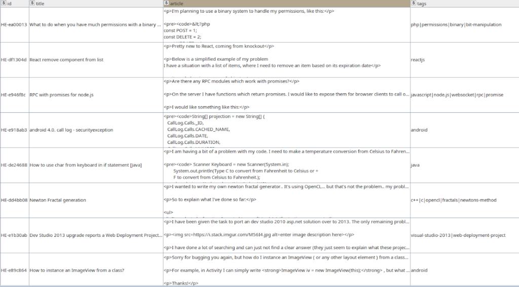
Figure *. The unprocessed data table.
With our nodes, we will train a model that will help us to automatically assign the labels for the questions and estimate this model with Jaccard coefficients and F_beta scores.
Data Processing for our Case of Multi-Label Classification
The original data went through simple preprocessing like removing HTML tags, then it was resampled to take the most frequent combinations of classes, so we will have a quite balanced data set. This way the data set used in the demo contains 23694 records. On the bar chart (see fig.1) you can see the distribution of tags combinations – here we have some major classes mostly including “javascript”, “HTML” and “SQL” tags, but the rest of the classes are more balanced.
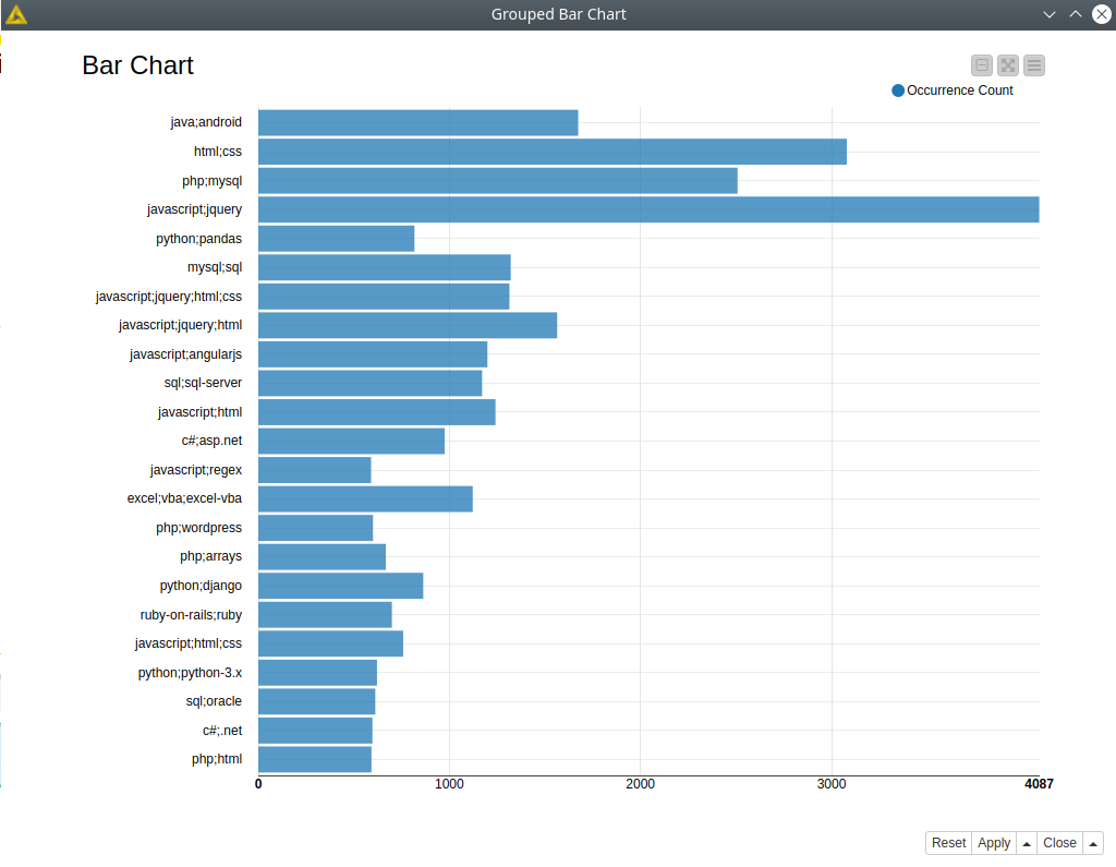
Figure 1. Barchart with class distributions.
This way we have 23 unique combinations of classes with multiple intersections and not-fixed number of classes for the intersections. Now we are good to go and split the data before training, we are going to use training, validation and test subsets. To sample them we are going to use two Partitioning nodes with stratified sampling option to keep the same ratio between the classes in all the subsets.
Model Training for Multi-Label Classification
First we need to get the BERT-based model from TensorFlow Hub or Hugging Face repository. To do this we need to use the BERT Model Selector node that comes from BERT by Redfield extension and is completely compatible with the Redfield NLP nodes.
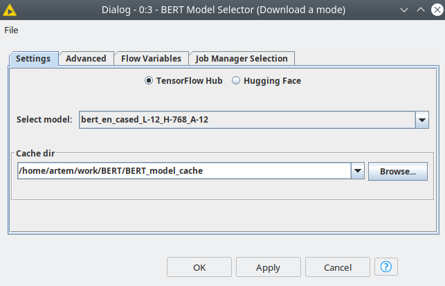
Figure 2. BERT Model Selector settings where a model can be selected and for its further usage.
Then the model will be downloaded from the repository and saved in the provided directory for further usage. This is the bare BERT that has been trained by a third party, now we need to build a small neural network on top of it and fine-tune this complex model. For this purpose, we are going to use BERT Multi-label Classification Learner.
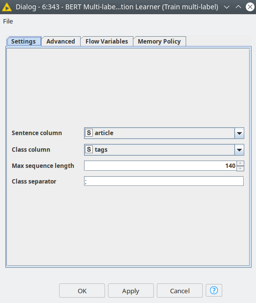
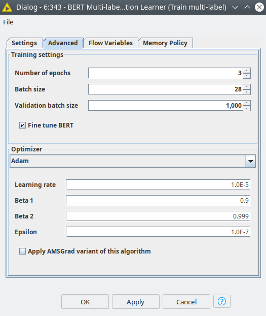
Figure 3. BERT Multi-label Classification Learner nodes dialog.
In the node settings the user is expected to select the column with text, a column with labels, and max sequence length – the expected length of the text that will be processed, usually, it is better to calculate a mean or median value for the corpus and use this value. In the Advanced tab, the optimizer and training settings can be set up. These settings are very similar to the BERT Classification node, and you can read more about it in our previous article on the Knime blog.
Model estimation
Once the training is over we can make it predict the labels for the test data set. In order to do this we need to use a node from BERT by Redfield extension – BERT Predictor – which is compatible with multiple BERT-based models.
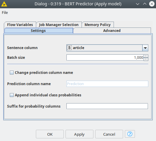
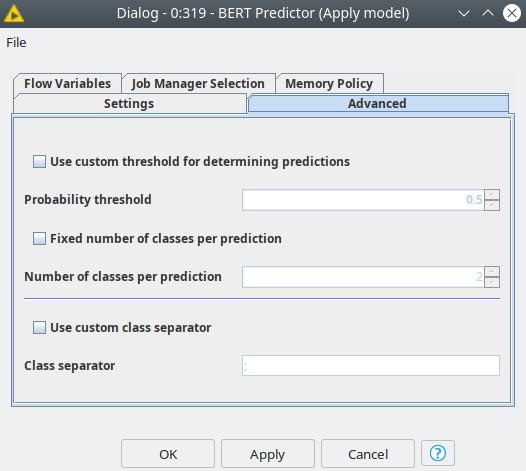
Figure 3. BERT Predictor node dialog settings.
In the predictor, you can define a probability threshold for a class assignment or fix the number of the assigned classes. By default classes with the highest probability will be assigned. Now we have the predictions, but the standard way of model estimation models like confusion matrix or calculation of recall and precision or other metrics is trickier than for simple one-label classification. The reason is that as long as we have several tags in the prediction we can consider multiple cases:
- All predicted tags matched the known tags – a perfect prediction.
- Some but not all of the tags match, or we have some extra incorrect tags assigned – a partial prediction.
- None of the assigned tags matched the known tags – an erroneous prediction.
In order to define the false negative, false positive, and true positive prediction we are going to calculate the Jaccard coefficient and based on its values identify the validity of the prediction. The Jaccard coefficient is a well-known metric that estimates similarity in many applications of data science: image recognition, market basket analysis, and multi-label classification tasks in general. All these calculations are encapsulated into Multilabel results visualization, this component also plots different model predictions estimations.
In total, we got only 328 out of 5735 misclassifications which is roughly 6%, about 70% (4046 out of 5735) were predicted correctly and about 24% were partially predicted. And based on the Jaccard coefficient where we assumed the values more than 0.5 to be true positives, less than 0.5 as false positive, and equal to 0 as a false negative. Then we were able to calculate precision, recall, and F_0.5. In that case, the model got quite high scores (see figure 4).
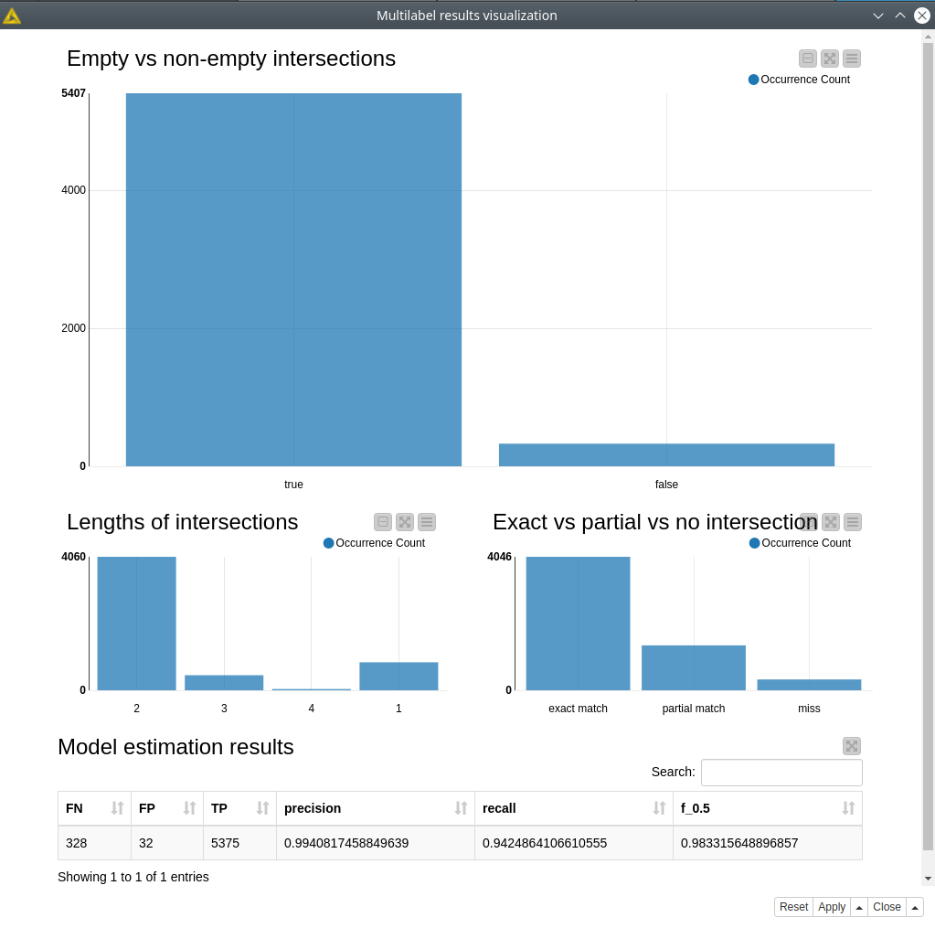
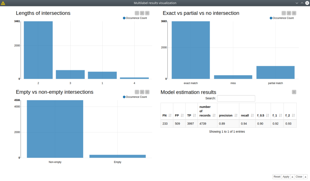
Figure 4. The dashboard with model performance estimation.
Conclusion
In this article, we have discovered how to solve the problem of multi-label classification without using code at all. That task is common for businesses where you might need to identify several aspects from customer reviews or complaints, identify the keywords for the document, define multiple groups for a product based on its description, etc. This task can also be easily scaled using the Knime server for the training process, where you might need a powerful GPU. Then you can process thousands of texts and get the dashboards with the prediction analysis similar to what we have built in our demo. Another use case for the Knime server is building a microservice where the text can be sent via REST API you can immediately get the prediction. In the latter case, you even do not need a powerful GPU-instance once your model is trained and ready for production usage.