


The data and its preparation
In this blog post, we are going to train multiple models to find the sarcasm detected in headlines. The data set that is used was taken from Kaggle, and it contains short headlines, a URL to the original source, and a label column with just two values for sarcastic and non-sarcastic headlines. The workflow is available here.
The data is represented as a set of JSON strings, so obviously we need to transform it to a Knime table. To do this we read all those lines with Line Reader, convert the strings to JSON objects, and parse them with JSON Path. Another thing we need to do to find sarcasm detected is to convert the class notation for the original 0 and 1 to “non-sarcastic” and “sarcastic”. That’s it, BERT-based classification models do not require any other preparation, they only need 2 things: raw texts and labels. Using the Bar Chart node we can we the distribution of classes (see fig. 1), fortunately, this data set is pretty balanced. And using the Text assessment component we can the statistics of the lengths of the texts. This information is useful to select a good value for a global BERT parameter – max_seq_length that defines how many tokens will be considered by the model.
WARNING: As long as BERT models can only be efficiently fine-tuned with GPU we highly recommend you to use CUDA compatible graphics card. Another issue is that BERT might require a lot of VRAM, this way please estimate the capabilities of your hardware and use Row Sampling node with a warning message to set up a reasonable number of samples your hardware can handle.
Then we need to prepare several datasets for training, validation, and testing of BERT models and a control data set that will be used later for training models on word embeddings. For this purpose, we use a set of consequent Partitioning nodes. Now we are set up for training.
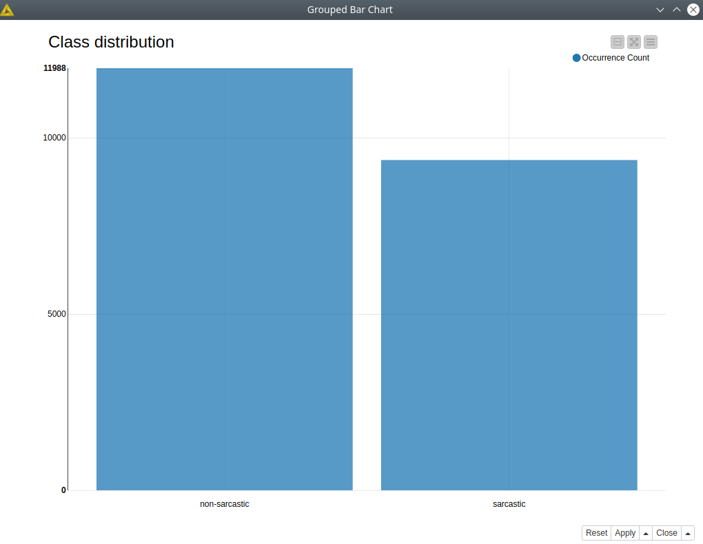
Figure 1. Distribution of classes.
Table of Contents
Training the BERT models
In the first part of the “sarcasm detected” experiment we are going to train two BERT-based models: one with BERT fine-tuning and one without. In the first case, we will fine-tune the whole huge model that includes BERT itself and the shallow classification neural network on top of it, in the latter case we will train the shallow neural network only. It may depend on the data and your expectation about the model’s predictive power, but in general fine-tuning, the whole model gives better results, however, it takes more time. So let’s see how it works in practice.
First, we need to get a BERT model from one of the repositories: TensorFlow Hub or HuggingFace. To do this we are using the BERT Model Selector node: we are going to take a BERT standard uncased model for English from TensorFlow Hub since our texts are lower-cased (see fig. 2). In the node dialog, you can also provide a path where you would like to cache your models, so you do not have to download them again next time.
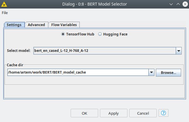
Figure 2. BERT Model Selector dialog.
Fine-tuning the whole model
First, we need to define the parameters of training: max_sequence_length this parameter defines how many tokens will be considered by the model. We are going to set this parameter to 16, and Text assessment helps us since we can see the statistics of text lengths of the texts. Having this value means that more than ¾ of our texts will be completely considered by the model. And the batch size for both models is set to 128 (you can change it depending on your hardware capabilities, it should not dramatically affect the model quality). These are the main global parameters that both models share.
Training BERT classifier with fine-tuning
Let’s first train a model with fine-tuning (blue box), this model will be trained in just 3 epochs, and we set the learning rate quite low 1E-4, the rest of the optimizer parameters are the default values. To do so we are going to use the BERT Classification Learner node, below you can see the dialog, where the user is only supposed to provide the settings for training with no code at all.
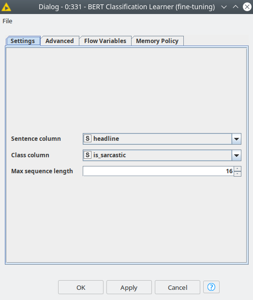
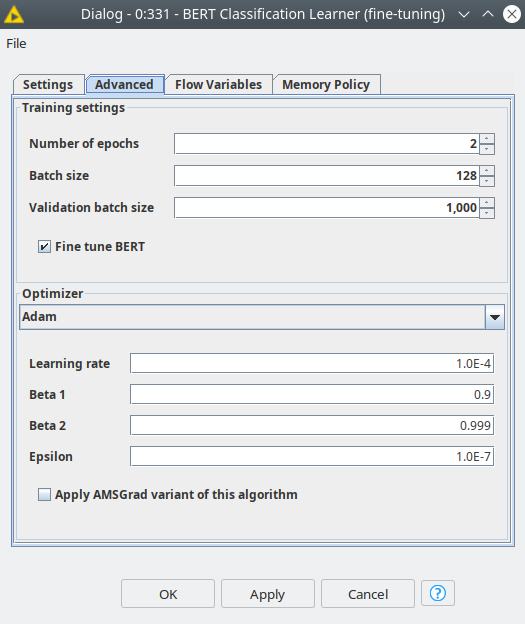
Figure 3. Settings of the BERT Classification Learner, showing settings for the case of fine-tuning the BERT classifier.
This node has 2 ports for data, the first one expects the training data set, the second one is a validation data set, but this is optional. However, it is extremely useful to provide a validation data set, then you can see if the model training goes fast or slow and if the model becomes overfitted. After training, we can see some information about the model, how it was evolving after each epoch of training (see fig. 4).
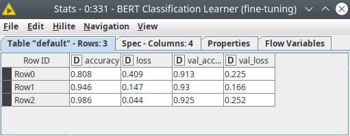
Figure 4. BERT classifier training with the fine-tuning report.
And we can see that actually, we could train just only for 2 epochs to get the best results for sarcasm detected, since after the 3rd epoch model started overfitting. Nevertheless, the model we got is quite good, let’s proceed and estimate its quality on the test data set. Now we need to feed the model to the BERT Predictor node (see fig. 5). In the settings we need to specify the column with the texts, also here we can set up the batch size – the number of records processed in one go, and some other settings.
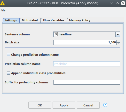
Figure 5. BERT Predictor node dialog.
And then to estimate the classification model we can use a standard Knime node – Scorer. And we can see that we got pretty good results: around 91% accuracy and 82% Cohen’s kappa (see fig. 6). And we did not even try to optimize any training parameters for the model or better balance the data set!
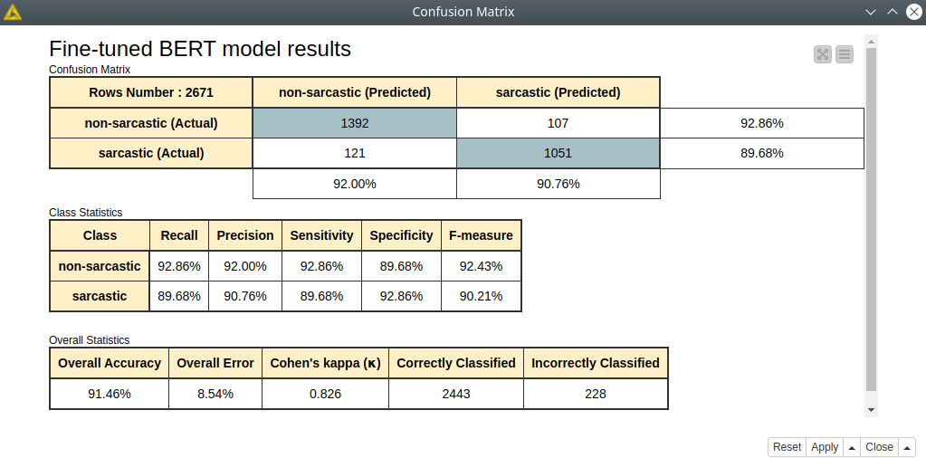
Figure 6. Fine-tuned BERT model quality assessment.
Training BERT classifier without fine-tuning
Just to compare, let’s also train a BERT model without fine-tuning to see the difference. We are going to change only 2 parameters for this case: the number of epochs = 8 and learning rate=1E-3, in order to try to get comparable results as for a fine-tuned model.
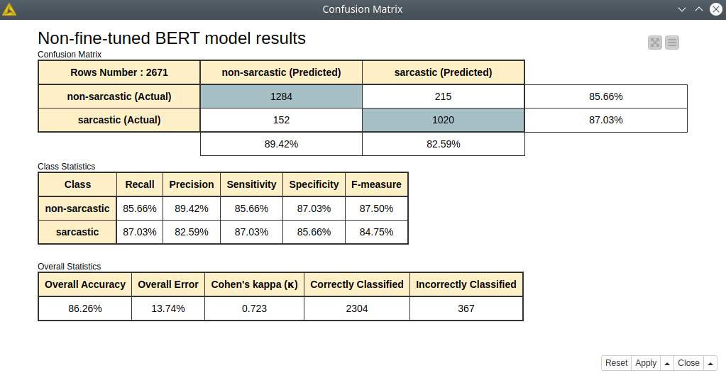
Figure 7. Non-fine-tuned BERT model quality assessment.
For this case we are getting slightly worse results, however, training even for more epochs took less time than for a fine-tuned model (fig. 7).
Embeddings learning case
Now let’s consider another use case of how BERT functionality can be used. As long as BERT itself can be considered as a huge encoder that translates texts into vectors, called embeddings, we can consider the embeddings as the features for other machine learning algorithms. In this demo we are going to demonstrate 3 use cases for how to use embeddings:
- Use embeddings as features to train other less heavy-weight models – Random Forest and k nearest neighbor.
- Use dimensionality reduction for embeddings for visualization.
- Use dimensionality reduction for embeddings to optimize the training for Random Forest and k nearest neighbor models.
Using embeddings with RF and kNN
To extract embeddings we are going to use the BERT Embedder node, which is compatible with both pink and grey color ports. This means that you can extract embeddings from both fine-tuned and non-fine-tuned models, we are going to take a look at both of these cases. First, let’s take a look at the BERT model without fine-tuning, so let’s just connect feed the model directly from BERT Model Selector to BERT Embedder, and we are going to use a control data set. The settings of this node are quite straightforward, you just need to select the column with the texts and specify max sequence length the same as for Learner (see fig.8).
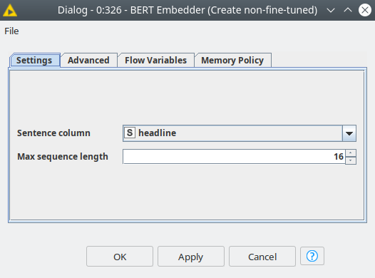
Figure 8. BERT Embedder node dialog.
As the output, the BERT Embedder returns a list of doubles, and the size of this collection is defined by the BERT you have picked in Model Selector. The model we used in this demo returns a vector with 768 numbers for each text. Then we unwind this collection with Split Collection Column node, prepare training and test data set out of control data set, and now we are ready to go with native Knime ML nodes. In this demo, we are going to use 2 well-known algorithms: random forest, the most popular tree ensemble algorithm, and kNN, which is based on calculating distances between the samples. We are also going to apply PCA in order to reduce the dimensionality from 768 to 3 so we can plot our sample on a 3D scatter plot.
We are going to take the default settings for the training settings, except that for the random forest we are going to set up the number of models = 300, and for k nearest neighbors k = 101.
First of all, training for both algorithms is way faster than even for the BERT model without fine-tuning – this is one of the benefits. You also do not need to use GPU to train these models. As we can see these results are much worse than even non-fined-tuned BERT classifier (see fig. 9). So there comes the tradeoff between accuracy and time of training the model. And looking at the PCA 3D projection (fig. 10) we can see that samples are evenly scattered, so no surprise it is hard to distinguish between sarcastic and non-sarcastic texts. Let’s see if we can improve the predictions using the same model based on fine-tuned embeddings.
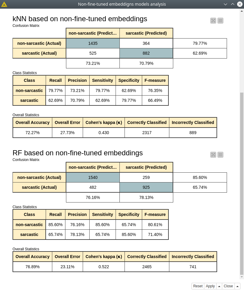
Figure 9. Random forest and kNN model assessment trained with non-fine-tuned embeddings.
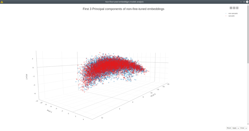
Figure 10. 3D scatter plot of first 3 principal components based on non-fine-tuned BERT model. Non-sarcastic samples are blue, sarcastic ones are red.
Using fine-tuned embeddings with RF and kNN
Now let’s connect to the BERT Embedder node, the model that we have fine-tuned, other settings remain the same. Then the algorithm is the same – split the List column, and use these features to train random forest and k nearest neighbors models. The settings for the model training are the same as for the previous case.
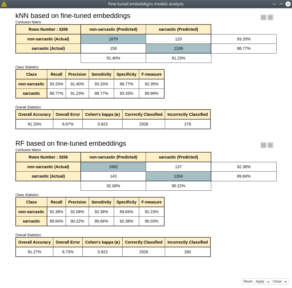
Figure 11. Random forest and kNN model assessment trained with fine-tuned embeddings.
The results we obtained are almost the same as we got for the BERT classification model (fig. 11). However, training and inference of kNN and random forest models take much less time. It does not require using GPU as well. This is a perfect case for the situation when you can train a BERT classifier once and then use it as an encoder that perfectly describes your data. This approach is very efficient for metric learning tasks, which implies using kNN, clustering algorithms, or any other distance-based algorithms.
Using principal components of fine-tuned embeddings with RF and kNN
And the last experiment for today – we are going to significantly reduce the dimensionality of the embeddings we are getting from BERT. For this purpose, we are going to use a very simple and well-known algorithm of principal components analysis (PCA). The benefits of PCA are that this algorithm is very fast, it can be reversed back to original data, the PCA model can be reused for new data and it has a native implementation in Knime. Of course, you are encouraged to try more sophisticated algorithms such as t-SNE or UMAP.
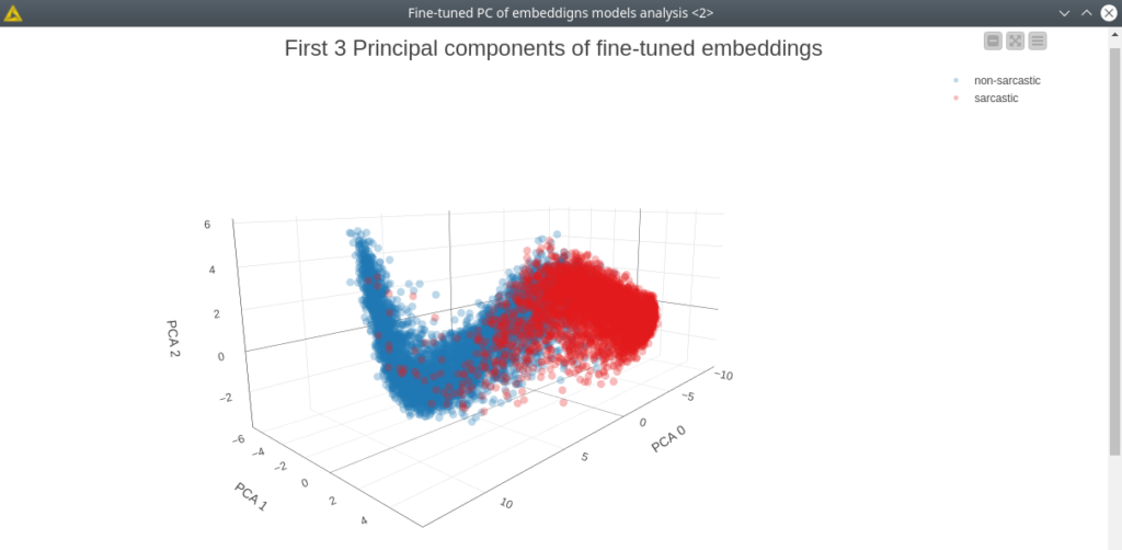
Figure 12. 3D scatter plot of first 3 principal components based on fine-tuned BERT model. Non-sarcastic samples are blue, sarcastic ones are red.
Looking at the 3D PCA projection (fig. 12) now makes everything clear what are the benefits of fine-tuning – the samples now scattered in two big clusters, obviously separating samples, in this case, is a much more simple task. In the settings of the PCA Apply node, we are going to take the first 10 principal components that will actually preserve 95% of the information. This way our gain here is that we significantly reduced the size of the data – 10 features vs 768 features in the original data set – hence we will reduce the time of training and inference of the models. So let’s train the same models with the same settings and estimate them. The settings for random forest and kNN are the same as in the previous example.
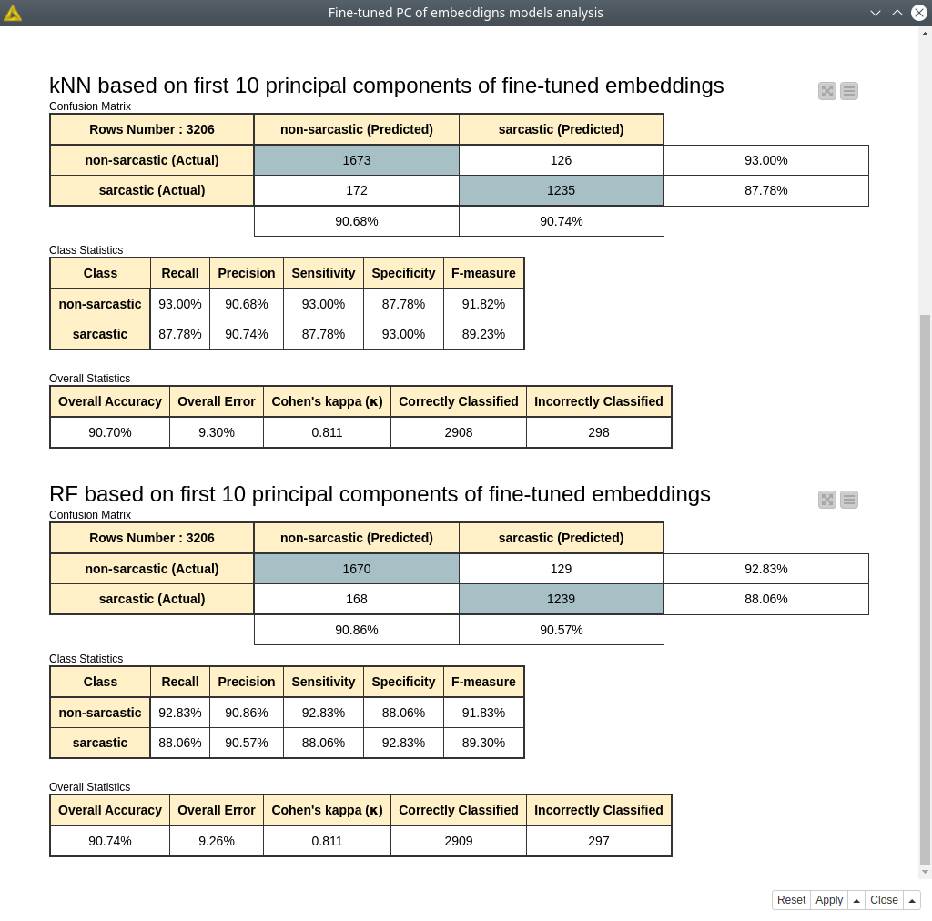
Figure 13. Random forest and kNN model assessment trained with 10 principal components of fine-tuned embeddings.
The models we got have a very small decrease (~1-2%) in accuracy, Cohen’s kappa, and other metrics compared to the previous cases: fine-tune BERT classifier and RF/kNN trained on fine-tuned embeddings (see fig. 13).
This is another good solution in case you are looking for a more optimized solution: train a BERT classifier based on a big enough data set once, apply PCA and save the model, then use the latter two models (BERT and PCA) to create features for training with kNN or random forest algorithms. And once you got a decent model you can just use BERT and PCA models just for feature engineering and then use these features to run kNN or random forest models to make predictions.
Sarcasm Detected with Machine Learning: Conclusion
In this blog post, we have reviewed several examples of using BERT embeddings: we have compared how the fine-tuning makes a significant difference in the models’ output, how other more simple algorithms can utilize the embeddings, how we can reduce the dimensionality of the embeddings in order visualize the data and optimize both training and inference processes.