
(as first published at knime.com)
In the last decade, NoSQL databases have become very popular. Neo4j is one of the leaders in the field of graph databases. It is a popular schema-less database with its own query language called Cypher and is perfect for storing relationships: logistics data, social network data, financial transactions, chemical reactions, and more.
In this article, we’d like to give you:
- An overview of the nodes that make up our Neo4j extension for KNIME Analytics Platform that enable you to access Neo4j databases and analyze the data in KNIME
- Demonstrate how the extension can be used for ETL, analysis, and visualization in KNIME
Our topic? Cocktails! We hope you enjoy the article.
What is Neo4j?
Neo4j does not have a strict schema, all the data stored there is presented as nodes and relationships. Nodes represent entities of any nature, while relationships represent any kind interactions and connections between entities. Both nodes and relationships have a label, nodes might have multiple labels (e.g. Person:Student, Person:Teacher), while relationships may have only one label (e.g. IS_A, KNOWS, WORKS_AT). The relationships are directed, so there is always a source node and a target node, and it can be the same node as well. This structure is really handy to deal with unstructured data, it gives a lot of benefits in case you are building a graph that includes data from multiple domains and describes the relationships between them.
Dataset
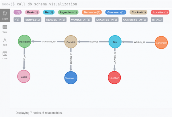
The dataset contains information about the cocktails, their ingredients, bars where these cocktails are served, bartenders who serve them, glassware, and more. The data were taken from Kaggle, however initially it was provided by Hotaling&Co.
We used this dataset as the data is general enough that everyone can quickly understand the benefits of representing the data as a graph. Our graph scheme is straightforward, see figure 1.
Overview of the Neo4j extension
There are three nodes in the extension, but this is everything we need.
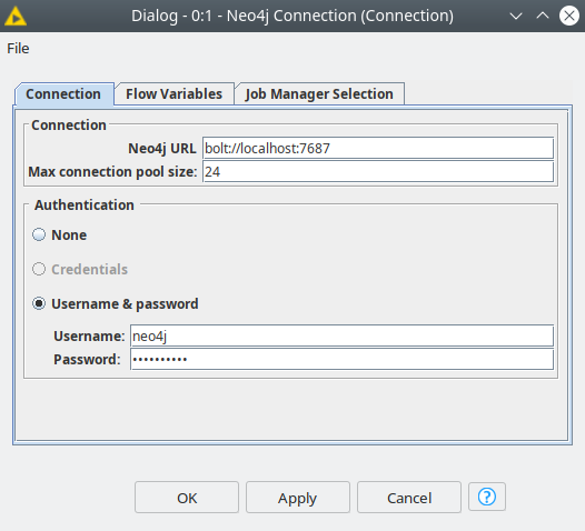
- Neo4j Connection — connects to the Neo4j instance via native BOLT protocol. The settings here are pretty straightforward:
- URL, username and password. You can also use KNIME credentials if you created them in the workflow.
- Max connection pool size — the number of connections to the database, by default it is equal to the number of available CPU threads.
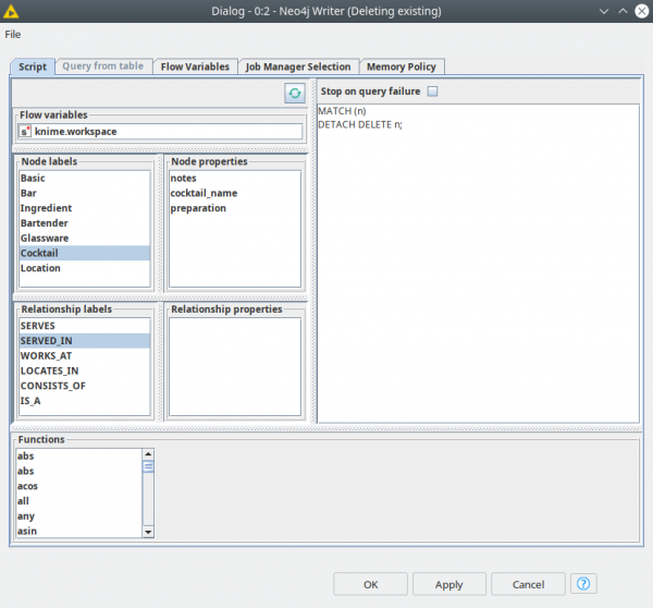
- Neo4j Writer — pushes data into the database. It has two modes:
- Script mode – script where the user provides a Cypher query. This query can be enriched with injections of node and relationship labels, their properties, Neo4j functions and flow variables — just double-click on one of them to inject into the script body (Figure 3).
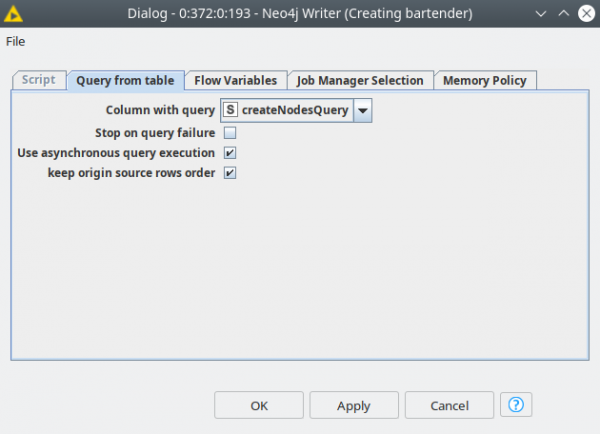
- Table mode – this mode is to run queries from the table. To use it you need to activate the dynamic port and feed the table with Cypher queries (String column) to the node. The dialog here is simpler, you just need to select a column with queries and the query execution mode: asynchronous or sequential. The first mode runs the queries in parallel batches, which is faster, however if the order of execution matters deactivate this checkbox (Figure 4).
Both modes support fault tolerant execution mode: “Stop on query failure” allows to skip the queries that could not run for any reason, the node will always execute if this checkbox is not active.
- Neo4j Reader — this node is used for data extraction from the database. Its dialog is similar to the Writer node; it also has the same modes: script and query from table. This node can match the data types between Neo4j and KNIME and can convert primitive types (String, Integer, Double, etc), dates and collections. Otherwise it is always possible to return JSON with “Use JSON output” checkbox, it can be useful if you want to extract a lot of complicated data structures.
ETL made easier with shareable components
The first and most tedious part is processing the data and populating the database. As dataset is not perfect we need to prepare the data. Essentially what we need to do is fix the column names, as these will be used as properties in the database and get rid of missing values of ingredients – as we don’t want to have cocktails in the database without ingredients. We have created a number of components to take care of these tasks. Let’s take a closer look at them.
- Look up KNIME Verified Components – a set of components developed by KNIME and the KNIME Community, verified by KNIME experts.
- Find out more about encapsulating functionality with components in this video What is a Component? on our KNIMETV YouTube channel.
Adjacency table creator with properties
This component has a dialog that asks you to define the columns for future source and target nodes. In the example shown in figure 2 we are going to create nodes for Bartender and Bar, where Bartender is a source and Bar is a target. In the second part of the dialog you can pick which column to be used to create source node properties.
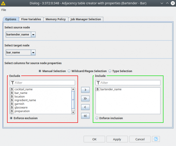
This component produces intermediate tables to be fed into the Node Creator and Node ID Matcher components. The three outputs are:
- An aggregated table for future source nodes with lists of consecutive future target nodes
- An aggregated table for future target nodes with lists of consecutive future source nodes
- Column names for future source and target nodes
Node creator
This node generates the Cypher queries for creating the nodes and their properties. Use the dialog to:
- Provide the labels for the future nodes separated by “:”
- Filter for the properties for the future nodes
- Customize the return clause for the Cypher query. By default it returns the node IDs that we are going to use further to create relationships between the nodes. However it could be something else, node property or collection, just refer to the node with alias “n”. This field can also be empty.
- Alternate for the apostrophe and quotation characters. Since we are building a query as a string problems could arise if we were to include string properties with values containing these characters. By default is a backtick (`). This way we can use this workaround to exchange the characters.
- Select the mode: CREATE or MERGE. The CREATE clause just creates something in the database (in this case a node). MERGE basically means MATCH or CREATE, this operation is more expensive, however it prevents duplicates.
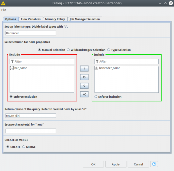
The output of the node is the table with the node selected properties and the Cypher queries built according to the settings. And this table is then fed to Neo4j Writer node, that can run multiple queries asynchronously.
Node ID matcher
This component does not have any configuration, so the user is only supposed to properly connect the inputs. The are four:
- The first port expects the output from the Neo4j Writer node which returns the node IDs of the source nodes
- The second port expects the aggregated table with target nodes and list of sources nodes (the second output of consequent Adjacency table creator with properties component)
- The third port expects the output from the Neo4j Writer node that returns the node IDs of the target nodes
- The fourth port expects a table with the column names for source and target entities (the third output of the consequent Adjacency table creator with properties component).
This component looks like a black box, but what it simply ungroups and joins the source nodes with target nodes. These joins are necessary to create the relationships between the nodes. We only need to perform joins here; afterwards all the relationships are stored in Neo4j.
Relationship creator
This component creates relationships. It is configured similarly to the Node creator component. You first select the columns with the IDs for source and target nodes. Next, provide a label for the relationship. CREATE or MERGE works similarly to the Node creator. Finally, the return clause is also similar to Node creator, however the default value is empty and the alias for the relationship is “r”.
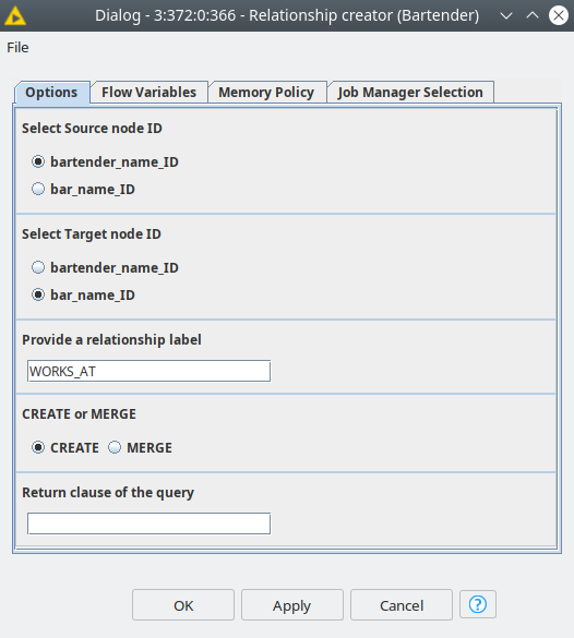
This node expects the output from Node ID matcher as input, and returns Cypher queries for creating relationships. This output should be fed to Neo4j Writer node.
Basic ingredients
There are two more sub-components inside our ETL component — Ingredient processing and Extracting basic ingredients. The idea here is to create a simple generalization of the components, since let’s say whisky is always whisky no matter what brand it is. We applied simple text processing methods to extract the basic ingredients .
Analysis
Once the data is uploaded to the database we get to the most interesting part — analysis. By using Cypher we now have well-prepared data for every case. In our example, we consider six cases, and all of them will be using the relationships of the entities — the power of graph. At the same time we are also going to use standard aggregation methods similar to relational databases.
Let’s take a look at each of the six use cases
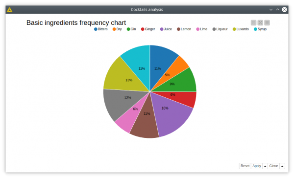
1. What’s the connection between the basic ingredients and the cocktails?
The query to investigate the connection is quite simple; it just gets 3 types of nodes and 2 types of relationships between them (equivalent to 2 joins in relational database). The aggregated data is processed in JKNIME to get the 10 most frequently used basic ingredients in cocktails, and visualized as a pie chart.
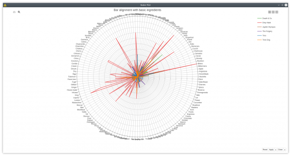
2. Aligning the bars to the basic ingredients
This case has a more complicated Cypher query, which adds bars to the previous query. We only want to look at the bars with more than 29 ingredients and visualize them as a radar plot. In this plot we can see that the ingredients in the right lower area are not used that much by these 5 bars. This kind of information might be useful if you want to serve more exotic cocktails and get an edge on your competitors.
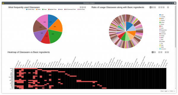
3. Connection patterns
Let’s add one more category for the analysis — glassware — and see if there are interesting connection patterns for cocktails that include both basic ingredients and glassware. We can plot a pie chart showing the usage frequency of glassware similar to the previous cases and plot the ratio of usage of basic ingredients per glassware with sunburst diagram. A heatmap shows which glassware is either used or not used at all with certain ingredients.
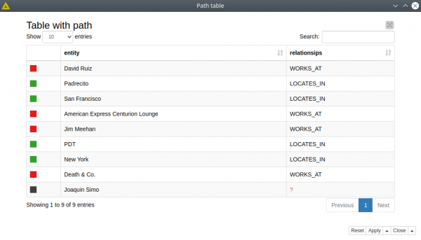
4. Graph-specific use case: traversal and path finding
Here we want to look for a connection between two bartenders — Joaquin Simo and David Ruiz. We want to restrict the relationships by their type: we are looking for other bartenders they might know or the bars they might be working at. We wrap all the step nodes and relationships into two lists, and then we unwind these lists with Ungroup node. Our visualization, built with the Path Table component shows us that these two bartenders have a mutual colleague who works in two bars in New York and San Francisco.
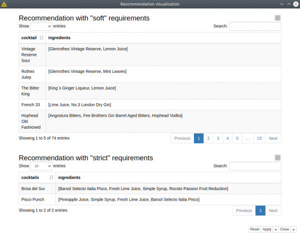
5. Recommending ingredients
What’s missing in our stock of ingredients to make some cocktails? The output is the table that contains cocktails and missing ingredients as recommendations (“soft” requirements).
We can also be more specific by using “strict” requirements if we want our cocktails to consist of all the ingredients we have.
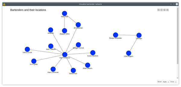
6. Bartenders working in multiple bars and their locations
First we look for the bartenders who work in more than one bar, second, we generate queries with the String Manipulation node to get the locations of the bars. As you can see it is possible to run multiple reading queries at the same time, and the results will be returned as JSON files. This helps to run different types of queries that might return distinct results. The JSON files are easily parsed with the JSON Path node. This is what we are doing inside the Visualize bartender network component, that shows the bartenders and their locations. Please note that we created a sub-graph in KNIME, since in Neo4j bartender and location nodes are not connected, they have bar nodes in the middle.
Wrapping up
In this blog post we demonstrated our Neo4j extension for KNIME Analytics Platform and worked with the databases to perform data migration – from table format to graph – and simple analytics based on the obtained data. Of course these use cases are not the only ones, and definitely not the most interesting. However understanding how to work with the concepts of graph databases are crucial before moving further.
Neo4j provides many internal tools for data processing, like native machine learning functions, integrations with other services such as Spark, and graph visualization. So there is a lot to explore, and the Neo4j extension provides a basic functionality to combine KNIME Analytics Platform and Neo4j.
The workflow we used in this blog article is available for you to download and try out for yourself from the KNIME Hub. Access the Cocktails graph with Neo4j workflow by Redfield from the KNIME Hub.
Redfield is a KNIME Trusted Partner.